LLMs of 4B and below on AI Agent Tasks

Why 4B and Below Is the Practical Size for Edge

Everything in this benchmark lives inside a hard constraint: an edge box has a fixed memory budget, and the model shares it with cameras, rule engines, dashboards, and everything else the deployment needs. On Jetson-class hardware, a 4B model at Q4 quantization takes roughly 2.5 GB just for weights, and KV cache grows on top of that. Go one tier up — 7B, 14B — and the weights alone crowd out the rest of the system, decode speed drops below what an interactive agent needs, and cost per deployed unit climbs out of the range where edge AI makes sense.

So the practical question is not “which model is smartest” but what can a 4B-and-below model actually do, once it runs where the devices are. Running where the data is changes what intelligence is worth: an agent that can read a sensor, write a rule, and confirm state on a local dashboard — without a round trip to the cloud — turns physical events into decisions in milliseconds, keeps private site data on site, and keeps working when the network does not. That is a different kind of intelligence from a large cloud model: less knowledge, but attached to the physical world, always available, and cheap enough to put everywhere.

This benchmark is our way of answering that question with numbers instead of impressions: the same 138 tasks, the same strict pass criteria, across every model small enough to be a real candidate for edge deployment today.

Evaluation Set and Pass Criteria

For this small language model benchmark we use the NeoMind Agent bilingual evaluation set: 69 regression cases, each rendered in Chinese and English, for 138 samples. Runs use NeoMind 1.2.3 with a 32K context window; verifiable sampling parameters are listed in the table below. The main leaderboard reports thinking-off results, and thinking mode is compared separately.

For every sample we check that the agent executed the expected commands, then a script verifies the post-run state assertions. We do not use an LLM judge.

Results: Small Language Models vs Larger Models

We present small on-device models alongside larger cloud models. All figures cover the full 138-task set (69 Chinese, 69 English). SFT results are discussed separately under Key findings and are excluded from the leaderboard. Qwen3.5-4B was run with two thinking-off sampling configurations: the model card’s recommended instruct setting (T0.7/P0.8) and an alternative test setting (T1.0/P0.95), with remaining parameters in the table. These are inference-time text-generation controls, not fine-tuning or weight changes; we list the two results separately so that parameter differences are not mistaken for model differences.

Multi-step and single-step columns split tasks by complexity. SFT results are discussed below. Abbreviations: T = temperature, P = top-p, K = top-k, minP = min-p, pres = presence penalty, rep = repetition penalty. Cloud rows have no on-device parameter count or GGUF quantization field; local quantization is labelled from the GGUF file actually served, and Gemma’s QAT means quantization-aware training with a Q4_0 file. The sampling column lists only parameters we could verify. Nanbeige4.2-3B completed 108 of 138 tasks and was stopped by its memory limit: it is the only dense-attention model in this set, its 32K KV cache is far larger than the hybrid-architecture models, and an earlier thinking run logged 839 context truncations before being voided — a full retest needs roughly 14 GB of memory for KV alone. Its task split is therefore not shown. A first official run scored 8.0% and was superseded by this one after a configuration fix; both runs are kept in the evaluation records.

Thinking mode helps, but by very different amounts

The gains are far from uniform. Spark-X2.6-1.7B rises from 43.5% with thinking off to 63.8% with thinking on, a 20.3-point gain (58.0% Chinese, 69.6% English), the best local result. Qwen3.5-4B scores 41.3% with thinking off using the Instruct setting T0.7/P0.8/K20/minP0/pres1.5/rep1.0, and 55.1% with thinking on using the model card’s reasoning-recommended T1.0/P0.95/K20/minP0/pres1.5/rep1.0; this gap includes both the thinking switch and the corresponding sampling change. Spark-X2.6-4B reaches 59.4% with thinking on, a 9.4-point gain over its 50.0% with thinking off and the best 4B result on device.

Where the gains land also differs by model. MiniCPM5-2B rises from 33.3% to 45.7% (+12.4 points; 49.3% Chinese, 42.0% English), but nearly all of it comes from single-step tasks — 58.2% on single-step against only 15.0% on multi-step — so what it buys is execution accuracy, not planning ability. Qwen3.5-4B is the opposite, with multi-step climbing from 17.5% to 41.4%. If your workload is mostly multi-step tool chains, thinking adds little for MiniCPM5-2B: its model card enables thinking by default, which this data supports for single-step work, but do not expect it to fix planning.

LFM3-1.7B gains the least from thinking (+4.3 points), and the cause is the test harness rather than planning ability. Each ReAct round emits 1,500–5,400 thinking tokens and often runs past 300 seconds; the platform’s thinking watchdog fired 36 times in this batch, and every cut-off voided that round, sending multi-step tasks into a cascade — its multi-step rate with thinking on is only 20.0% against Spark-X2.6-1.7B’s 50.0%, with failures concentrated on the planning chain. In other words, 47.1% is closer to a floor imposed by this harness than a ceiling on what it can do; with a more generous timeout on your side it may have room left.

LFM2.5-2.6B and Gemma-4-E2B are absent from the chart because their thinking switch did not take effect in this run: the on and off runs took essentially the same time, and their differences (+1.5 and +1.4 points) fall within noise.

The cost is the reasoning itself. With thinking on, the model must generate a reasoning trace before answering, so per-task latency rises. We suggest reading 63.8% as the ceiling when you are willing to trade time for pass rate, not as a default configuration; how much extra waiting it adds has to be measured on the target device.

40 multi-step and 98 single-step samples; the thinking-off column uses the standard configuration. MiniCPM5-2B’s thinking-off row is its historical run, with the split recomputed on the same criteria.

Decode speed on Jetson Orin NX

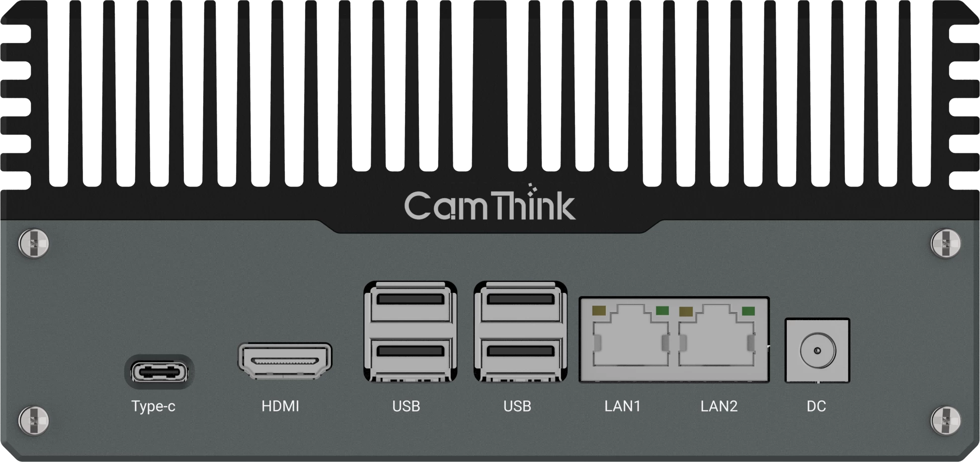
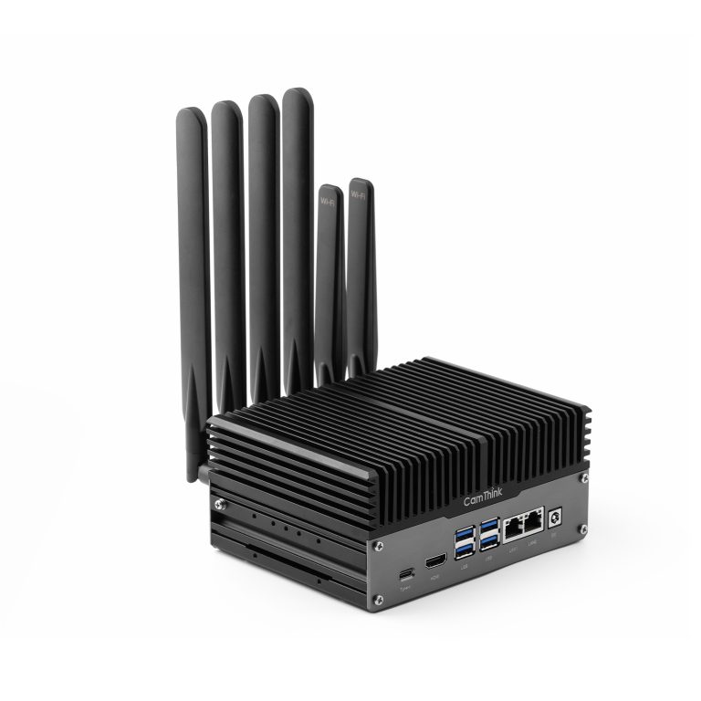
To add a device-side performance view, we measured single-stream decode speed and long-context behaviour for the models in this article on Jetson Orin NX. We also describe this Jetson Orin NX based edge AI box on the NG4500 product page. The test report covers one 8GB Orin NX module board and one 16GB Orin NX system; the two devices measured identical GPU specifications and agreed within 2% on overlapping data, so the results below are useful for NG4500 deployment sizing. Single-stream decode speed measures generation throughput, not agent task pass rate.

On this Jetson Orin NX test, LFM3-1.7B decoded at 49.0–49.3 tokens/s, among the faster local models we tested. On long context, we measured decode speed from about 1K to about 120K tokens of depth: LFM3-1.7B (256K native context) falls from 48.8 to 28.6 tokens/s, keeping about 59% of its speed, and still delivers 20.1 tokens/s at 240K depth. Spark-X2.6-1.7B and Spark-X2.6-4B retain about 61% and 57% at 120K. LFM2.5-2.6B drops to 13.5 tokens/s, and MiniCPM5-2B decays the hardest, down to about 4 tokens/s at 120K — worth noting for long-document use.

On memory, Liquid AI’s published LFM3 tests report roughly 1.6 GB of KV cache at 128K tokens, below the Qwen3.5-4B (4.3 GB) and MiniCPM5-2B (5.6 GB) it compares against. This lines up with our measured speed decay: as context grows, LFM3 keeps both memory pressure and speed loss comparatively contained, leaving room for longer agent tasks on memory-constrained devices. The 128K memory figures come from official tests with different settings than our Jetson measurements; actual usage still depends on device, inference framework, and quantization.

On concurrency, the report measured aggregate throughput at 8 parallel streams: MiniCPM5-2B about 183, Spark-X2.6-1.7B about 131, LFM3-1.7B about 125, LFM2.5-2.6B about 92, and Spark-X2.6-4B about 81 tokens/s — a starting point for estimating concurrent capacity.

Data from “Jetson Orin NX LLM Inference Performance Test Report” v1.2 (2026-10-27 to 10-29, covering the 8GB module board and the 16GB system); llama-server, Q4 quantization, full GPU offload, q8 KV unless noted; overlapping data across the two devices agreed within 2%. Long-context steps are a fresh prefill plus 64 decoded tokens; 8-stream figures are aggregate throughput. Spark-X2.6-4B has a single single-stream measurement, 18.4 tokens/s.

2B-class models closing in on larger ones

On the same strict criteria, DeepSeek-flash and GLM-5.3 reach 81.2% and 76.8% and still lead the local models. The gap is narrowing, though: Spark-X2.6-1.7B with thinking on reaches 63.8%, ahead of Qwen3.5-4B with thinking (55.1%) and even Spark-X2.6-4B with thinking (59.4%), the best 4B result. At the same time, models such as Spark-X2.6-4B and Qwen3.5-4B already run offline on device and show practical value on some agent tasks. We expect future 2B-class models to close in on what today’s larger models achieve on AI Agent work — not just the 4B tier in this article, but the leading cloud models as well — bringing more capability into smaller hardware budgets. This is an expectation about the trend, and still needs follow-up measurement.

Key Findings

1. A small lead is not a stable win

In this small language model benchmark, Spark-X2.6-4B scores 50.0% and Qwen3.5-4B 51.4% at T1.0/P0.95, a 1.4-point gap; Spark-X2.6-1.7B scores 43.5% and LFM3-1.7B 42.8%, only 0.7 points apart. Across 138 tasks these gaps are enough to shortlist candidates, but not enough to decide a deployment ranking on their own. We also weigh task type, running cost, and parameter settings before calling a model suitable for a real workload.

2. Sampling parameters change results substantially

On the same T4 machine we tested Qwen3.5-4B at T0.7/P0.8/K20/minP0/pres1.5/rep1.0 for 41.3%; changing only temperature to 1.0 and top-p to 0.95 lifted it to 51.4%, a 10.1-point gain. We also saw LFM2.5-2.6B move from 24.6% under a wrong configuration to 36.2% at T0.1/K50/rep1.1, and LFM3-1.7B from about 20% to 42.8% at the same settings. Neither LiquidAI model card lists top-p, so we do not invent a value. Sensitivity varies by model; we recommend publishing the sampling configuration alongside any score.

3. AI Agent workloads hinge on multi-step planning

With thinking off, the two 1.7B models score similarly overall but differ in strength: Spark-X2.6-1.7B passes 27.5% of multi-step tasks against LFM3-1.7B’s 17.5%, while LFM3-1.7B is slightly ahead on single-step tasks (53.1% vs 50.0%). If your agent typically has to look something up, call a tool, and then confirm state, we would start with Spark. Thinking mode widens that gap further — Spark-X2.6-1.7B rises to 63.8% overall — so it can serve both as a lightweight default and as a switchable higher-accuracy mode.

LFM3-think does take noticeably longer to respond, which is a trade-off to weigh. A single thinking turn emits roughly 1,500–5,400 tokens, and the wait comes mostly from generating that reasoning. On low-power edge devices or in interaction-heavy scenarios that demand immediate response, this matters. We suggest judging task pass rate and response time together before enabling thinking.

Timeouts deserve particular attention. LFM3-1.7B with thinking ran on a T4 machine, where 28 samples took more than 5 minutes each, 12 took more than 10 minutes, and the slowest ran close to 18 minutes. In production environments that need stable response times, a timeout should count as a failure: our pass criteria already count incomplete tasks as failures, but if your upstream timeout is shorter, your real availability will be lower than the leaderboard suggests. Before deployment, measure the end-to-end latency distribution rather than just the average.

4. Supervised fine-tuning can also raise task completion

In the historical records, MiniCPM5-2B with SFT scored 40.6% strict pass against 33.3% for the un-tuned version (+7.3 points). This SFT run was an initial attempt, without systematically built training data or an optimized training pipeline for the target agent tasks. We expect more thorough task-data design and training optimization to yield larger gains; that judgement still needs measurement. Because both runs belong to an earlier batch, SFT is discussed separately and excluded from the leaderboard.

Choosing a Model by Deployment Constraints

Parameter count is no longer the sorting axis: a 1.7B model with thinking on beats 4B models with it off. The real trade-offs come down to three things — how much memory the device has, how complex the tasks are, and what a failed task costs.

If pass rate comes first, choose Spark-X2.6-1.7B with thinking on. At 63.8% it is the best local result, at the cost of longer waiting; confirm on site that this is acceptable.

If you need a larger footprint, the reason is usually no longer pass rate. A 1.7B model with thinking on already outranks this tier, so picking a 4B model is mostly about capabilities outside this evaluation set, such as multimodal input or longer context. For those needs, Spark-X2.6-4B with thinking on (59.4%) is the highest-scoring 4B option, with Qwen3.5-4B next (55.1% with thinking on, 51.4% with it off), but verify against the capability you actually need.

If memory is tight or you can only run thinking off, prefer 1.7B. With thinking off the 1.7B and 4B results are close (43.5% vs 51.4%), so picking the smaller model to fit the memory budget is the better trade.

One special case: for long documents and long context, LFM3-1.7B is the only choice — 256K native context and still 20.1 tokens/s at 240K depth, which no other model here matches; with thinking on it reaches 47.1%, a smaller gain than the other models show.

Decode speed and usable context are selection criteria in their own right — and they are where sub-4B models earn their place. Across this set, decode speed at short context tracks model size closely: the 1.7B–2.6B tier runs 34–49 tokens/s on Jetson Orin NX, while Spark-X2.6-4B manages 18.4. Usable context separates them even harder: LFM3-1.7B has 256K native context and keeps about 59% of its speed at 120K, the Spark pair keeps 57–61%, and MiniCPM5-2B decays to roughly 4 tokens/s at 120K. Nanbeige4.2-3B shows the other side of the trade: competitive pass rate, but a dense-attention KV cache that grows quickly with context. If your agent has to stay interactive on modest hardware, the smaller-and-faster column of the table is the one to read first.

Two closing reminders. The leaderboard answers whether a task can be completed; it does not cover latency or concurrency — both depend on device, inference backend, and load, and must be validated on your target hardware. And the cost of a failed task tends to be underestimated: a wrong deletion or a wrong configuration usually costs far more than waiting a little longer, so workloads with that profile should favour the higher-pass-rate configuration. Before deploying, always pin the model version, quantization, context length, and sampling parameters on the target device, and re-run a task set that matches your own devices, rules, and agent flow.

Limits: a Selection Ruler, Not an Acceptance Test

This small language model benchmark measures how well models complete NeoMind platform operations; it cannot replace acceptance testing against your own site data and production load.

At 138 tasks, one percentage point is about 1.4 tasks, so gaps within 4–5 points should not be read as differences in ability. And the leaderboard records a model × configuration, not pure model capability — changing sampling parameters alone can move one model by more than 10 points, so ranking without the configuration is meaningless.

We do not report cross-model latency comparisons here: the models were run on different hosts, so the speed numbers are not comparable; tasks that could not be completed count as failures in our criteria, and if your upstream timeout is shorter, real availability will be lower than the leaderboard suggests.