Two sites can have the same number of cameras and require very different edge hardware. Eight low-frame-rate streams running one detector are not the same workload as eight high-resolution streams running detection, tracking, secondary classification, recording, and multiple event outputs.
The useful sizing question is not “How many cameras does this box support?” It is “Can this hardware sustain this complete pipeline under the site’s busiest expected conditions?”
Size the Pipeline, Not the Camera Count
Start with one representative stream, measure the complete workload, then scale it with realistic concurrency and operating headroom. Camera count remains part of the calculation, but it cannot stand in for codec, resolution, frame rate, model input, tracking, event logic, storage, and integrations.
| Workload Layer | What to Record | Why It Changes Capacity |
|---|
| Video input | Codec, profile, resolution, FPS, bitrate, GOP | Decode and memory traffic vary by stream profile and scene complexity. |
| Inference | Model, input size, precision, interval, batch behavior | Different networks consume different compute and memory. |
| Analytics | Tracking, zones, classifiers, re-identification, rules | Post-processing can become a significant part of the pipeline. |
| Outputs | Events, snapshots, clips, overlays, database and API calls | Encoding, storage, and integration work continue after inference. |
| Operations | Peak concurrency, restart behavior, updates, monitoring, headroom | A lab maximum leaves little room for scene spikes or maintenance. |
Start with the Video Workload
Build a stream profile for every camera group. Cameras with the same nominal resolution may still differ in codec profile, frame rate, GOP structure, bitrate, or motion level. Test the exact production stream where possible. A sample file that has been transcoded on a laptop no longer represents the original decode path.
Do not assume the main stream is always required. A substream can lower decode and memory load when it preserves the smallest useful target. The IP camera compatibility guide explains how to check stream access and image usefulness before sizing begins.
Add the Model and Tracking Load
Record the actual model artifact, input dimensions, precision, inference interval, and any batching. Then add the work around it: preprocessing, object tracking, zone tests, secondary classification, temporal rules, and event deduplication. A detector that runs comfortably alone may behave differently once tracking and business logic are active.
Use the same event density expected on site. Empty-scene tests can understate post-processing load, while a crowded entrance, busy loading bay, or full parking area may produce more objects and more downstream work per frame.
Account for Decode, Memory, Storage, and Outputs
GPU or accelerator utilization is only one signal. Watch decoder use, CPU load, system and device memory, memory bandwidth, thermal behavior, network throughput, storage writes, and queue depth. If the application records clips or annotated video, include encoding and disk activity in the test.
Integrations also matter. Event delivery to a VMS, MQTT broker, webhook, database, or central platform can create bursts and retries. A sizing result is incomplete if it stops at the model output tensor.
Benchmark One Stream Before Multiplying
- Run decode only and confirm the stream is stable.
- Add preprocessing and the candidate model at the intended input size.
- Add tracking, zones, classifiers, and event persistence.
- Enable snapshots, clips, overlays, storage, and external outputs.
- Repeat with representative busy scenes and difficult lighting.
- Increase concurrent streams in controlled steps while logging resource use and dropped work.
Keep the test repeatable. Note software versions, model build, device power mode, ambient conditions, and each stream profile. This makes a later hardware or pipeline comparison meaningful.
Apply Operating Headroom
Do not select the point where a demo first reaches the target stream count. Leave room for scene variation, reconnect bursts, model updates, telemetry, and normal software overhead. The right margin depends on the operational consequences of overload and on how quickly the site can recover.
Define the failure policy as part of sizing. Decide whether the system may reduce inference frequency, drop noncritical overlays, queue events, or must continue every pipeline at the requested rate. That policy determines what “capacity” means for the project.
Choose One Box or Several Site Nodes
One larger node can simplify management, but it also concentrates network traffic and failure impact. Several local nodes may fit sites with separate buildings, constrained links, or camera groups that must continue independently. Physical network topology often settles this decision before peak compute does.
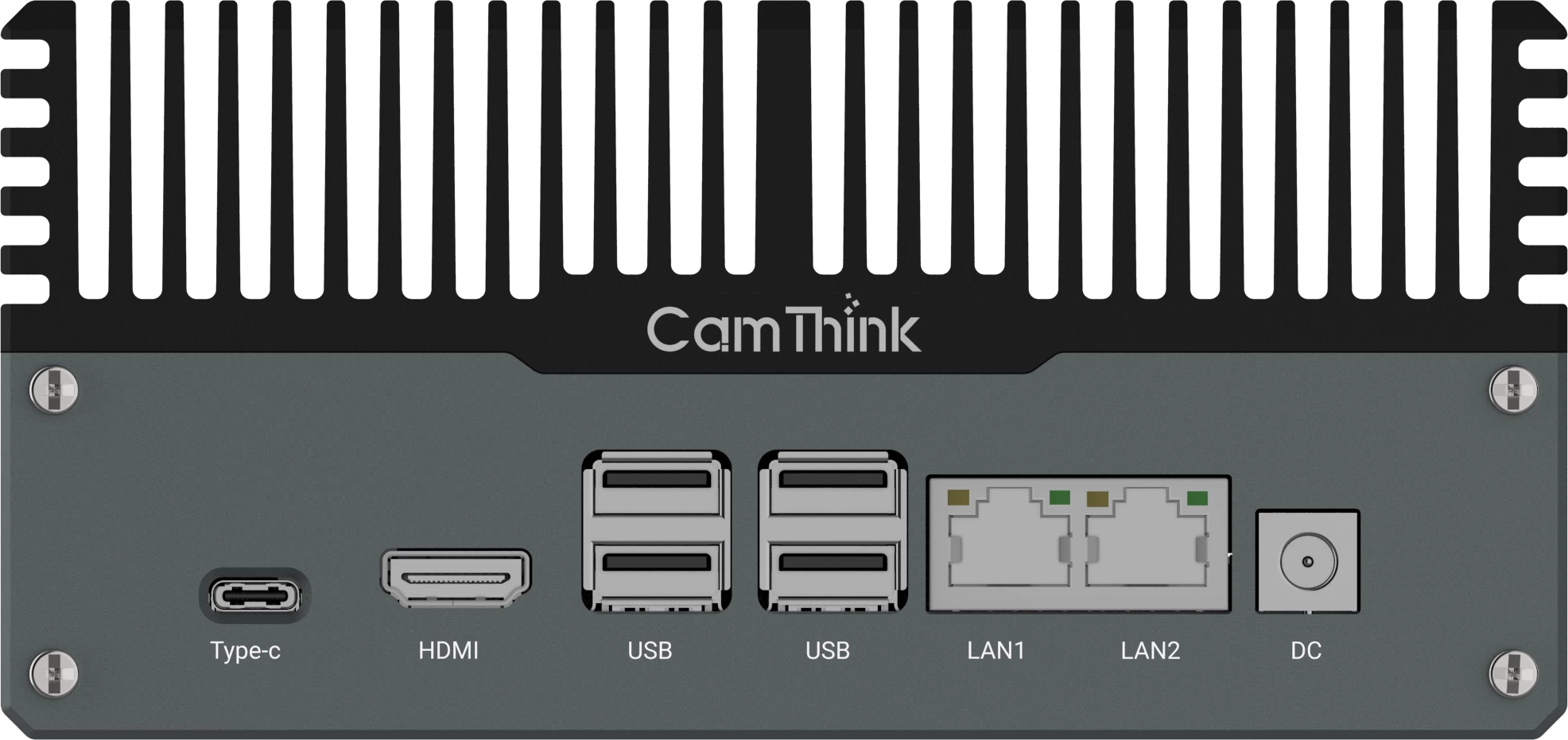
When streams are already stable and the workload is known, the NeoEdge NG4500 provides Jetson Orin Nano and Orin NX configuration paths for evaluation. If you share the stream profile, model, tracking, and outputs, ask CamThink to review an NG4500 sizing benchmark.
Use an NG4500 Evaluation Matrix
| Workload Pattern | Evaluation Direction | What Must Be Proven |
|---|
| Lower-resolution streams, one compact model, light event output | Begin with an Orin Nano configuration | Decode stability, target recall, sustained utilization, and margin |
| Mixed streams, tracking, or several event rules | Compare Orin Nano and Orin NX configurations | Memory use, crowded-scene load, output bursts, and recovery |
| Larger models, secondary inference, or heavier pipelines | Begin evaluation on an Orin NX configuration | End-to-end throughput and thermal stability with all services enabled |
| Separate buildings or constrained camera networks | Compare one central box with multiple site nodes | Network load, fault domains, maintenance, and aggregate cost |
This matrix is a starting point, not a published channel-count promise. The selected module and number of nodes should follow a measured pipeline test.
- Camera count grouped by codec, resolution, FPS, and bitrate
- Representative footage from normal and peak conditions
- Model files or model family, input size, and inference interval
- Tracking, classifiers, zones, and temporal event rules
- Required snapshots, clips, overlays, storage, and retention
- VMS, MQTT, API, database, or central management outputs
- Site network topology, thermal environment, and recovery policy
With those inputs, a PoC can answer a specific capacity question instead of repeating a generic camera number.